R and graphics devices on Mac and Windows

Today, I tried to plot some spatial data in R and observed some weird behavior. Digging deeper revealed some interesting differences between plotting in R with different operating systems. My work computer is a Mac and my private computer runs Windows, but I still use it primarily for work (for private life – and, well, work too – I have a tablet). Long story short, running the exact same R code on both computers, produces very different image files, because the operating systems use different graphics devices. This post summarizes the differences I found.

The problem

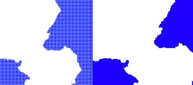
My first approach was running my code on the Mac and saving it via RStudio. Since that took a lot of time (and looked a little weird), I gave it a shot and tried running the same code on my Windows machine with the exact same settings saving it in RStudio as a png. Here are zoomed in versions of the two initial images side-by-side (zoom was done by hand and is not exact).

The left one comes from the Mac, has a size of 1.7MB, and a weird coloring that shouldn’t look like this. The Windows version on the right only has a size of 26KB and seems fine. At least when it comes to color. A careful comparison with the screenshot below of the shapefile in ArcGIS reveals that the border outline isn’t perfect either.

The “literature review“

I found other people complaining about slow plotting of spatial objects on a Mac, and this person observed a similar weird behavior (but not as extreme) for plotting on Mac vs. Windows in general (but no real solutions there). Most helpful in understanding the role of the graphics device for plotting issues in R on Mac was this site, which provides examples for the same plot with different graphics devices on a Mac. I will do something similar here, just for Mac and Windows output.

The data

The data is an Austrian regional statistical grid shapefile that consists of 1,353,322 individual polygons, each representing a 250m x 250m cell covering all of Austria. I guess the main issue is: it has a lot of individual polygons. Here is a screenshot of the Shapefile in ArcGIS, zoomed into the same general area as in the images before.

The code I started with

I wanted to simply plot the geometry, but fill the polygons in blue and make the border transparent. This was my original code that I ran on both machines. On Windows it produced the expected output, on the Mac it didn’t.

library(sf)

#download and unzip data
download.file("http://data.statistik.gv.at/data/OGDEXT_RASTER_1_STATISTIK_AUSTRIA_L000250_LAEA.zip", "OGDEXT_RASTER_1_STATISTIK_AUSTRIA_L000250_LAEA.zip")
unzip(file.path(".", "OGDEXT_RASTER_1_STATISTIK_AUSTRIA_L000250_LAEA.zip"), exdir=getwd())

#import data
AT_poly <- st_read("STATISTIK_AUSTRIA_L000250_LAEA.shp")

#plot data
plot(st_geometry(AT_poly), border="transparent", col="blue")

The png() options

To change the graphics device for a png file, we can use png() and specify the type and antialias options. Each will produce a slightly different output. On a Mac you get the options type = c("cairo", "cairo-png", "Xlib", "quartz") and here are some more details from the png() help.

type: character string, one of "Xlib" or "quartz" (some macOS builds) or "cairo". The latter will only be available if the system was compiled with support for cairo – otherwise "Xlib" will be used. The default is set by getOption("bitmapType") – the ‘out of the box’ default is "quartz" or "cairo" where available, otherwise "Xlib".

antialias: for type = "cairo", giving the type of anti-aliasing (if any) to be used for fonts and lines (but not fills). See X11. The default is set by X11.options. Also for type = "quartz", where antialiasing is used unless antialias = "none".

On Windows you get the options type = c("windows", "cairo", "cairo-png") and the help offers this additional information.

type: Should be plotting be done using Windows GDI or cairographics?

antialias: Length-one character vector.
For allowed values and their effect on fonts with type = "windows" see windows: for that type if the argument is missing the default is taken from windows.options()$bitmap.aa.win.
For allowed values and their effect (on fonts and lines, but not fills) with type = "cairo" see svg.

The output for choosing different options

Default settings (“windows” vs. “quartz”)

 png(filename="plot1.png", width 3000, height = 2700)
plot(st_geometry(AT_poly), border='transparent', col='blue')
dev.off() 

On Windows this is the same as choosing type = "windows".

 png(filename="plot1.png", width 3000, height = 2700, type = "windows")
plot(st_geometry(AT_poly), border='transparent', col='blue')
dev.off() 

On (my) Mac this is the same as choosing type = "quartz".

 png(filename="plot1.png", width 3000, height = 2700, type = "quartz")
plot(st_geometry(AT_poly), border='transparent', col='blue')
dev.off() 

Now the default settings with antialias = "none".

 png(filename="plot2.png", width 3000, height = 2700, antialias = "none")
plot(st_geometry(AT_poly), border='transparent', col='blue')
dev.off() 

Again, on Windows this is the same as choosing type = "windows".

 png(filename="plot2.png", width 3000, height = 2700, type = "windows", antialias = "none")
plot(st_geometry(AT_poly), border='transparent', col='blue')
dev.off() 

And also again, on (my) Mac this is the same as choosing type = "quartz".

 png(filename="plot2.png", width 3000, height = 2700, type = "quartz", antialias = "none")
plot(st_geometry(AT_poly), border='transparent', col='blue')
dev.off() 

Type “cairo”

png(filename="plot3", width 3000, height = 2700, type = cairo)
plot(st_geometry(AT_poly), border='transparent', col='blue')
dev.off() 

png(filename="plot4", width 3000, height = 2700, type = "cairo", antialias = "none")
plot(st_geometry(AT_poly), border='transparent', col='blue')
dev.off() 

Type “cairo-png”

png(filename="plot5", width 3000, height = 2700, type = "cairo-png")
plot(st_geometry(AT_poly), border='transparent', col='blue')
dev.off() 

png(filename="plot6", width 3000, height = 2700, type = "cairo-png", antialias = "none")
plot(st_geometry(AT_poly), border='transparent', col='blue')
dev.off() 

Conclusion

png() options		Mac		Windows
type	antialias	Quality	Size	Quality	Size
default	default	Worst	1.4MB	Ok	31KB
default	“none”	Ok	171KB	Ok	31KB
“cairo”	default	Good	31KB	Good	172KB
“cairo”	“none”	Good	31KB	Good	31KB
“cairo-png”	default	Good	43KB	Good	43KB
“cairo-png”	“none”	Good	43KB	Good	43KB

Using type = "Xlib" on the Mac kept giving me error messages.

The output differs between the different options as well as between the operating systems. Also the file sizes differed a lot. The file sizes provided are always for the entire image and not just the zoom. The biggest problem were the default settings for the Mac that produced a bad quality image that was also quite large. For code that is supposed to run on both operating systems type = "cairo" with antialias = "none" seems to be the best choice.

Are you wondering how the images would look if we wouldn’t draw the filling, but the borders and tried to plot them at the same resolution? It would obviously be a little screwed up, since the resolution wouldn’t be high enough to display the data correctly. Here is that comparison.